Prof. Moritz Diehl, Jakob Harzer, Katrin Baumgärtner
Modelling and System Identification (MSI) is concerned with the search for mathematical models for real-life systems. The course is based on statistics, optimization and simulation methods for differential equations. The exercises will be based on pen-and-paper exercises and computer exercises with python.
Course language is English and all course communication is via this course homepage.
If you have any questions regarding the exercises/lectures, please send an email to the tutors, syscop.msi@gmail.com
Lectures. The lectures will take place on Mondays, 8:30 - 10:00 a.m in Building 101, HS 026 and Wednesdays, 8:30-10:00 a.m. in Building 101, HS 036. If you cannot attend, you may watch the lecture recordings, see below.
Exercises. The exercise sheets include both pen-and-paper exercises as well as programming exercises using python. Exercise sheets can be handed in before the lecture on Monday, 8:30 or put into the Mailbox in front of room 00-075 in the ground floor of building 101 before. Programming exercises are handed in via Github Classrooms (more on that below). You have one week to work on the sheet and you might work in groups of at most three students.
Exercise Sessions. During the exercise session, the tutors disscuss the exercise solutions. Afterwards there is room for questions on the current exercise sheet.
- Group 1: Wednesday, 14:15 - 15:45, SR 00-031, Building 051, Premnath
- Group 2: Thursday, 10:15 - 11:45, SR 01-009/13, Building 101, Yizhen
- Group 3: Thursday, 14:15 - 15:45, SR 03-026, Building 051, Adithya
Written material. The lecture closely follows the script, which can be found below:
- Lecture notes on Modelling and System identification: PDF
If you missed the first lecture, you can pick up a printout of the script in Building 102, in the cupboard in front of room 00 075.
Please note that we do not cover Chapter 8.4. Additional material that covers some of the lecture contents:
- A script by Johan Schoukens (Vrije Universiteit Brussel, Belgium), which can be found here.
- The textbook Ljung, L. (1999). System Identification: Theory for the User. Prentice Hall. This book is available in the faculty library.
Summary Slides of the Course Organization
Final Evaluation and Microexams
Please make sure you register for both the MSI Exam and the MSI Studienleistung!
The final grade of the course is based solely on a final written exam at the end of the semester. The final exam is a closed book exam, only pencil, paper, and a calculator, and two handwritten double-sided A4 sheets of self-chosen formulae are allowed. It will take place on 21.03.2024, 14:00 -16:30.
Each exercise sheet gives a maximum of 10 points. Three microexams written during some of the lecture slots give a maximum of 10 exercise points each. In order to pass the exercises accompanying the course (Studienleistung), one has to obtain at least 50% of the maximum exercise points in each of the three blocks:
- Block 1: Exercises 1 - 3 + Microexam 1 (total 40 points) - Summary of points in Block 1
- Block 2: Exercises 4 - 6 + Microexam 2 (total 40 points) - Summary of points in Block 2
- Block 3: Exercises 7 - 10 + Microexam 3 (total 40 points + 10 Bonus Points) - Summary of points in Block 3 (without Ex10)
In a microexam, you will have 45 minutes for 20 multiple-choice questions on the lecture and exercises of the respective block.
To prepare for the written exam, check out the exams from previous semesters: 2019, 2018, 2015, 2014. (Please note that these exams contain questions on Appendix C of the MSI script, which is not covered in this year's lecture)
Solution video for the 2018 exam
Additionally, we will offer a Q&A Session on Thursday, 14.03, 10:00-12:00, Building 101, Room SR 01-016/18.
Lectures and Microexams
| Monday, October 16 | Introduction Lecture |
| Wednesday, October 18 | Lecture |
| Monday, October 23 | Linear Algebra Tutorial |
| Wednesday, October 25 | Lecture |
| Monday, October 30 | Statistics Tutorial |
| Wednesday, November 1 | No Lecture |
| Monday, November 6 | Lecture |
| Wednesday, November 8 | Lecture |
| Monday, November 13 | Lecture |
| Wednesday, November 15 | Lecture |
| Monday, November 20 | Lecture |
| Wednesday, November 22 | Lecture |
| Monday, November 27 | Lecture |
| Wednesday, November 29 | Microexam 1, 8:30 - 9:10, lecture from 9:15 |
| Monday, December 4 | Lecture |
| Wednesday, December 6 | Lecture |
| Monday, December 11 | Lecture |
| Wednesday, December 13 | Lecture |
| Monday, December 18 | Lecture |
| Wednesday, December 20 | Microexam 2, 8:30 - 9:10, lecture from 9:15 |
| CHRISTMAS BREAK | |
| Monday, January 8 | Lecture |
| Wednesday, January 10 | Lecture |
| Monday, January 15 | |
| Wednesday, January 17 | Lecture (on Modelling Temperature Profiles below Icy Roads) |
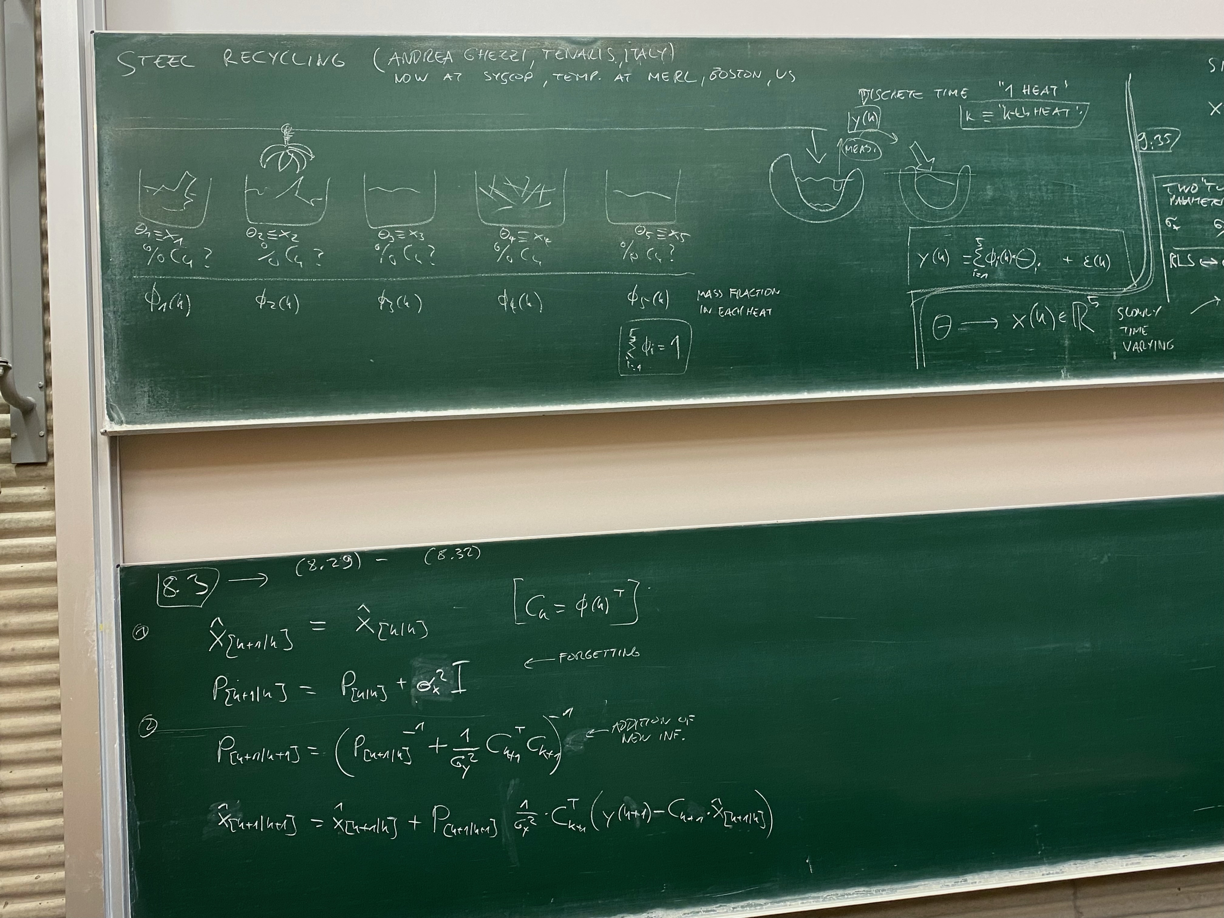
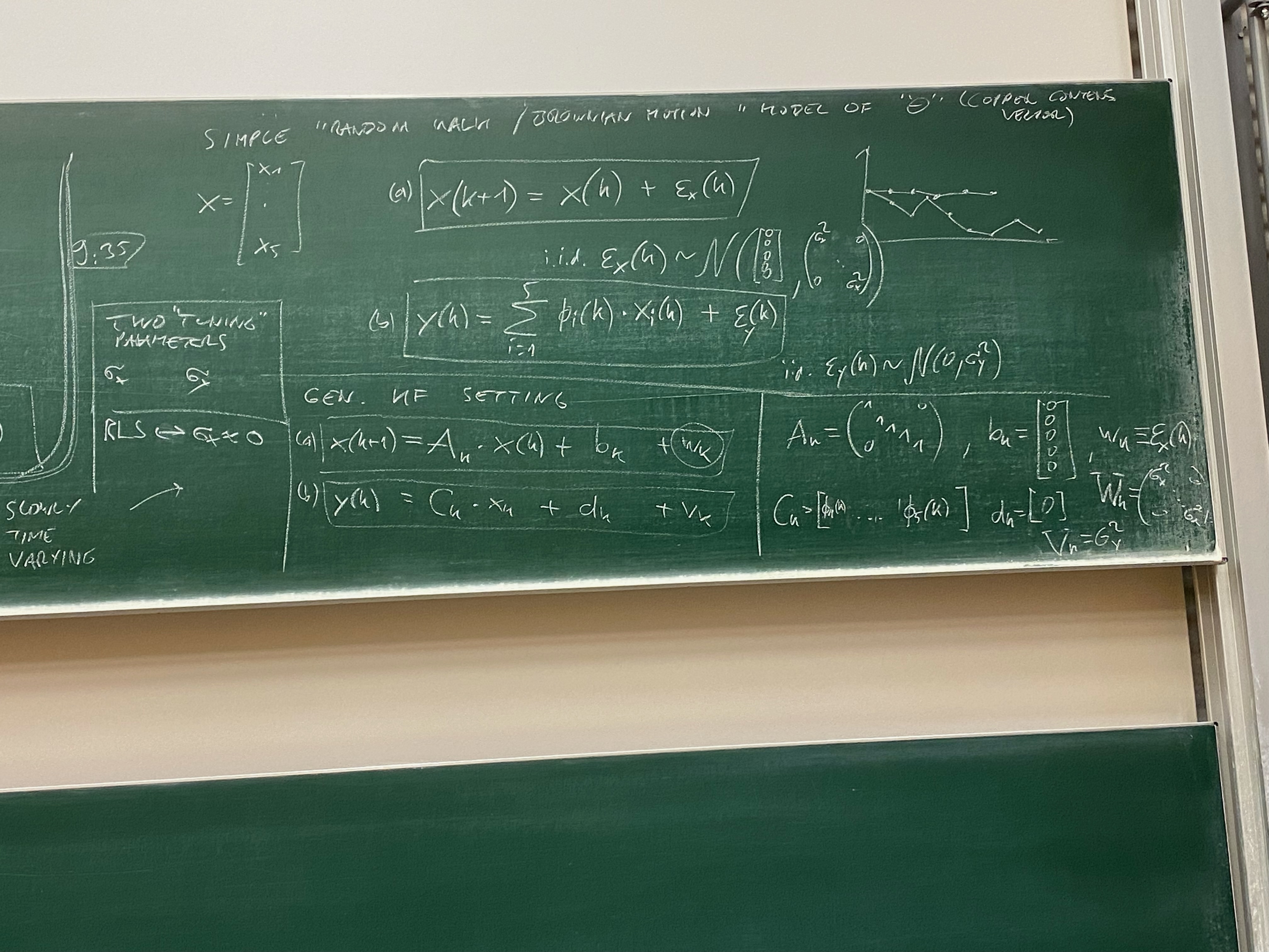
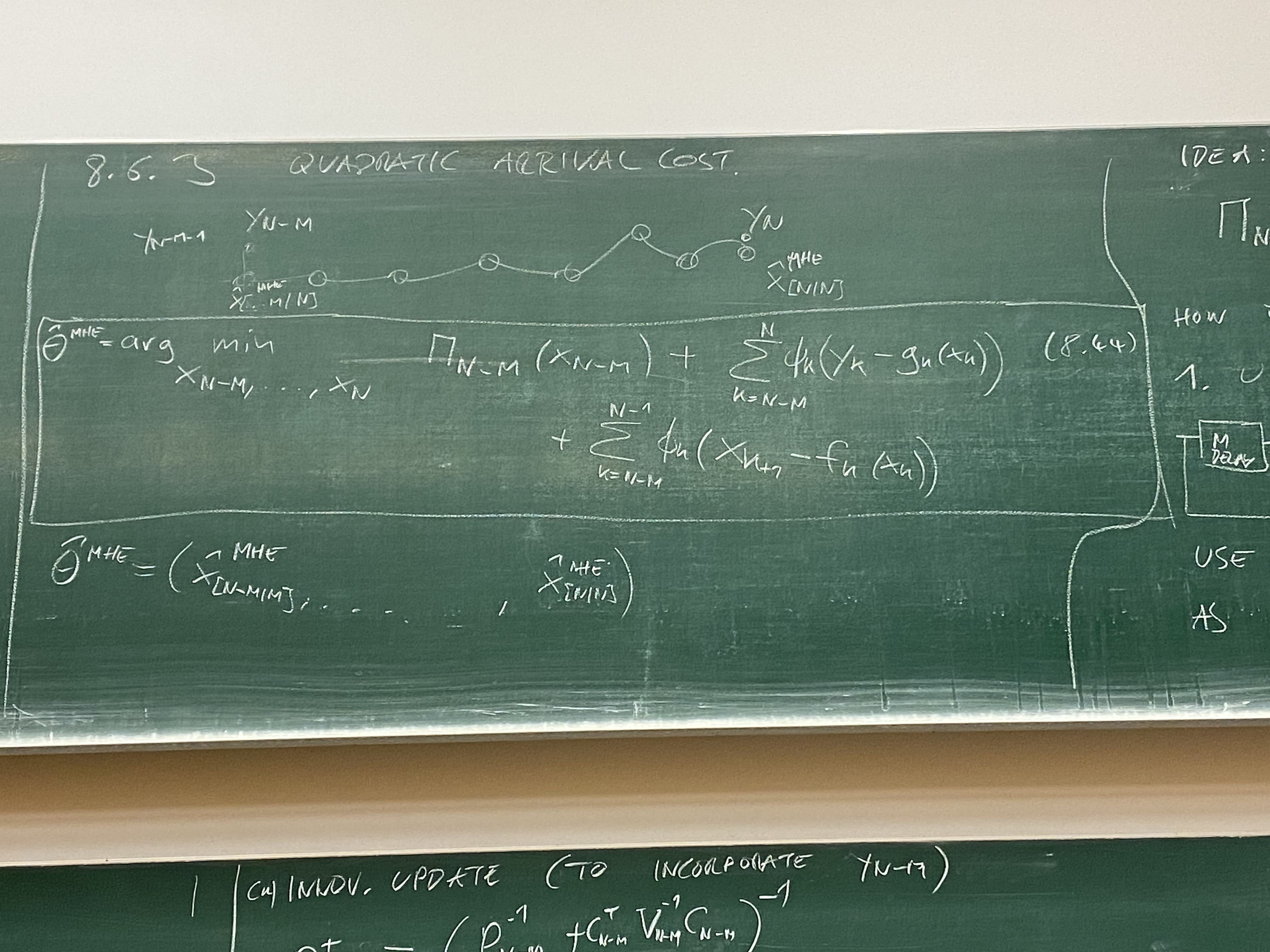
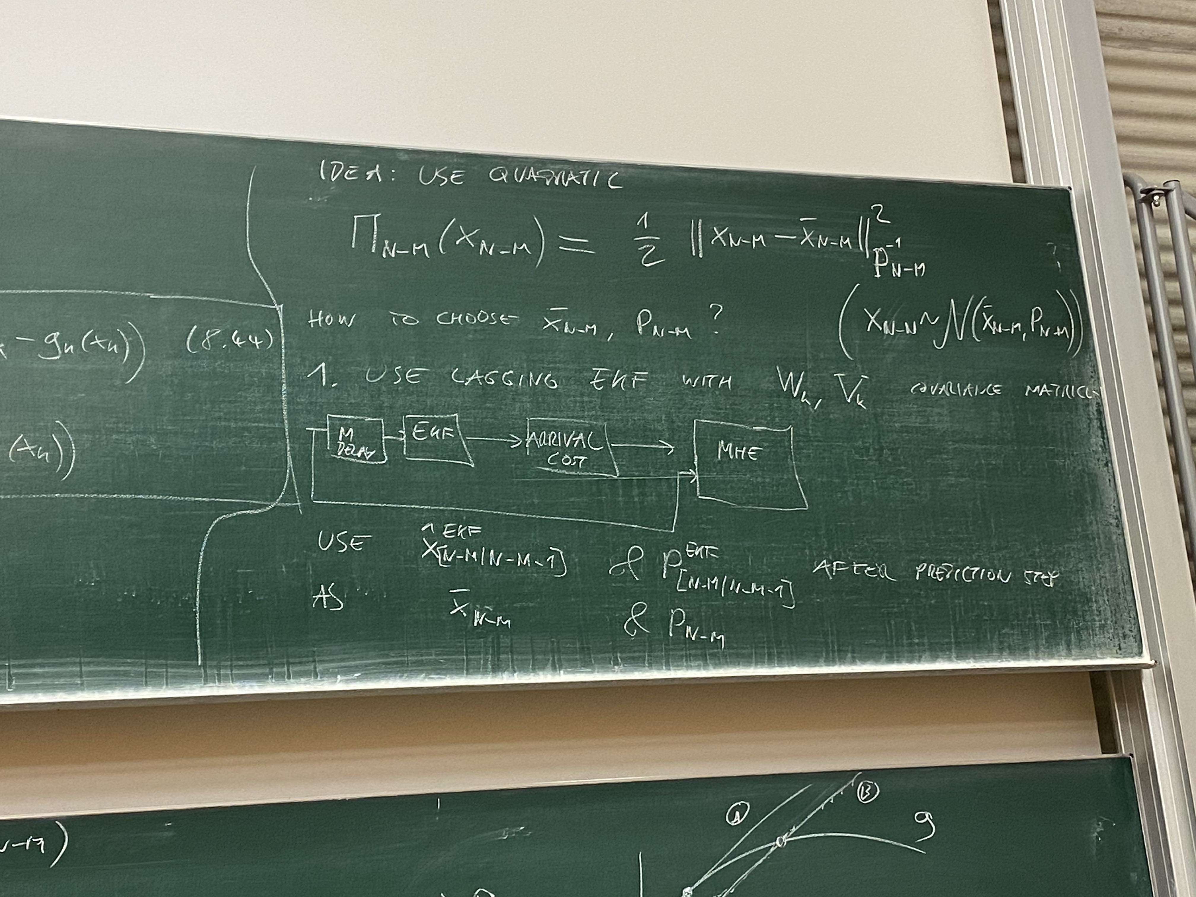
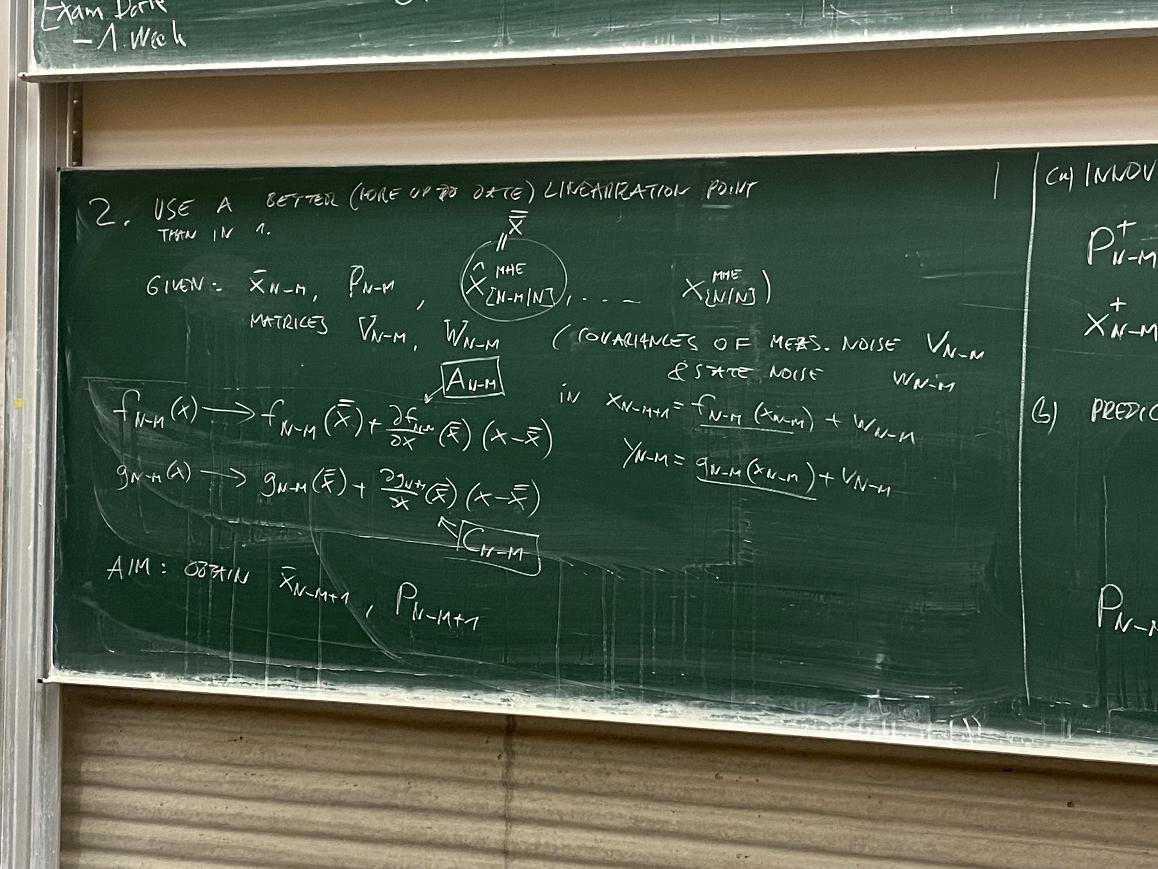
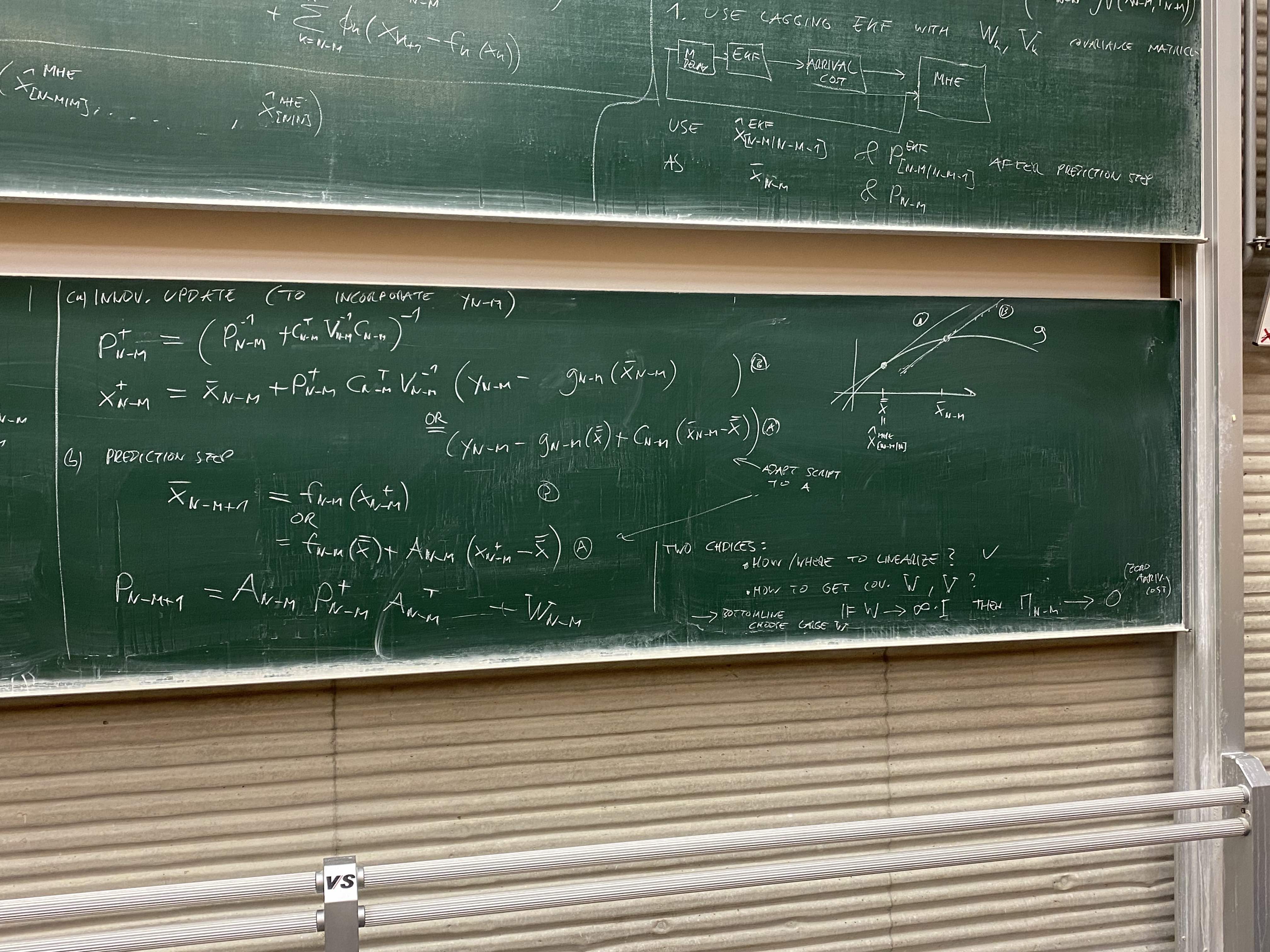
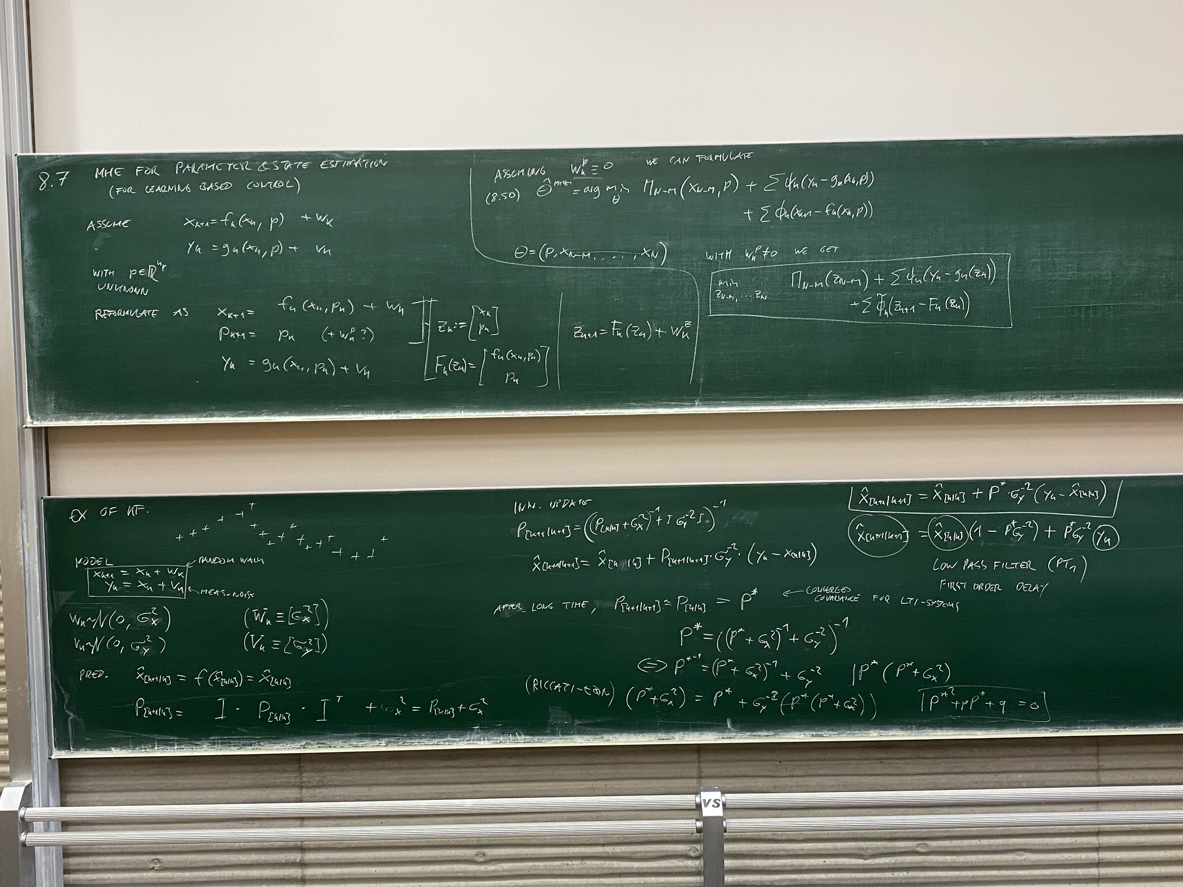
| Monday, January 22 | Lecture on Quadratic Arrival Cost in MHE and KF Example. Blackboard Photos: , IMG_8532.jpg, IMG_8533.jpg, IMG_8534.jpg, IMG_8535.jpg, IMG_8536.jpg |
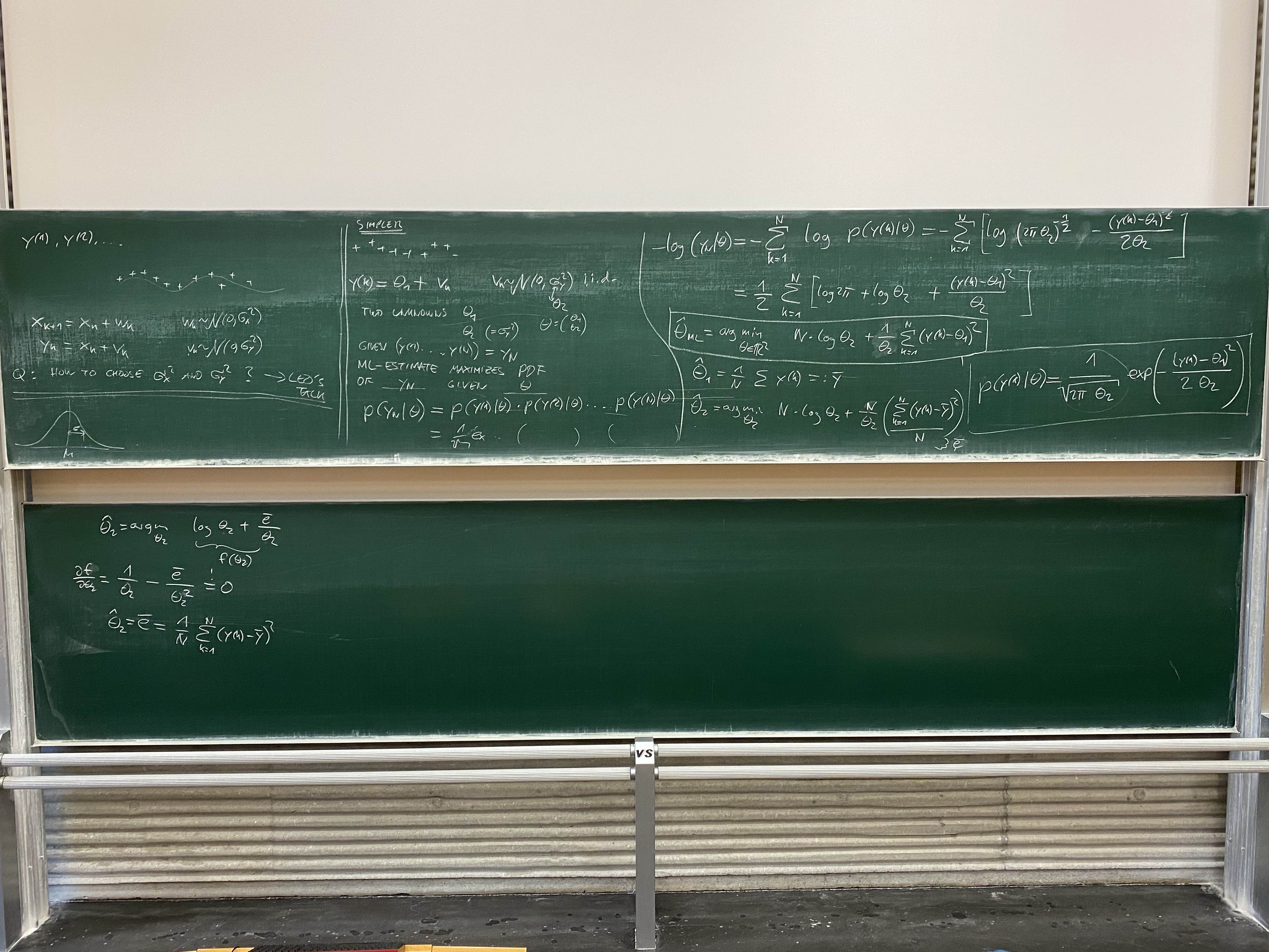
| Wednesday, January 24 | Talk by Wadi Abdurahim, Blackboard Photo on ML estimation of mean and variance: IMG_8537.jpg |
| Monday, January 29 | Talk by Leo Simpson, slides |
| Wednesday, January 31 | Microexam 3, 8:30 - 9:10, Talk by Moritz Berger afterwards |
| Monday, February 5 | Summary Lecture + Coffee |
| Wednesday, February 7 | Lecture: Past Exam Solution |
Tutorials
In the first weeks, there is no mandatory exercise sheet, but if you don't feel too confident about your linear algebra and statistics skills, you might want to check out these tutorials that cover the basics needed for the MSI course.
- Python Tutorial - for more information see the paragraph below
- Linear Algebra Tutorial
- Statistics Tutorial
In the first weeks, we will discuss these tutorial also in the lecture and the exercises.
Exercises Sheets
Github Classroom To distribute, collect and grade your coding exercises, we utilise Github Classroom. This service provides, for your exercise team, a Github repository for each exercise. If you have never worked with Git before, here we have linked a tutorial.
To use Github Classroom, every students need a github account. If you don't have one, or don't want use your private one, feel free to create a fake account just for this course. To identify your coding score with you immatriculation number, please register both your immatriculation number and your Github profile with us here. OTHERWISE YOU WILL NOT GET POINTS FOR YOUR CODING EXERCISES.
The exercise workflow looks as follows:
- Accept the exercise for your team above.
- Clone the exercises locally onto your computer.
- Work on the exercise, by executing the scripts
Check your solutions by running
pytest
in the console.
- Commit & push your solutions
- The same tests (with slightly different input data) are rerun on the server.
Python For the programming exercises we use Python. To work on the exercises please make sure to have Python installed on your system.
Python Installation
Here is a short guide on how to set up Python along with the IDE VS Code. If you already have Python installed on your system or want to use another IDE, feel free to skip to bullet 4.
- Install Python for your operating system
- Install VS Code
- Install the Python Extension for VS Code
- Install the required python packages:
- Start a terminal
Type and press enter:
pip install numpy scipy matplotlib pytest
Python Tutorial Notebooks
For people who do not know Python or want to refresh their knowledge, we provide a series of Jupyter notebooks to give you an introduction to data science programming in python. More resources, such as video tutorials for Python can be found online.
Download and unzip the Tutorial Notebooks into a folder of your choice
Open the folder in VS Code (File -> Open Folder)
Open the first Notebook by going through the file tree (notebooks/1-basics/PY0101EN-1-1-Hello.ipynb)
Lecture Recordings
| date | topic | chapters |
| October 18 - October 20 | Lecture 1: Introduction + Resistance Estimation | 1-1.2 |
| October 24 - October 28 | Lecture 2: Resistance Estimation + Statistic Basics | 1.2.2-2.3 |
| October 24 - October 28 | Lecture 3: Random Variables + Statisitical Estimators | 2.3-2.4 |
| October 31 - November 4 | Lecture 4: Resistance Estimation Revisited | 2.5-3.1 |
| November 7 - November 11 | Lecture 5: Optimization Basics + Linear Least Squares | 3.1-4.2 |
| November 7 - November 11 | Lecture 6: WLS + Ill-posed Problems | 4.3-4.4.1 |
| November 14 - November 18 | Lecture 7: Statistical Analysis of WLS | 4.5-4.7 |
| November 14 - November 18 | Lecture 8: Maximum Likelihood Estimation | 5-5.1.1 |
| November 21 - November 25 | Lecture 9: MAP Estimation + Recursive LLS | 5.2-5.3.2 |
| December 5 - December 9 | Lecture 10: Cramer Rao Bound (the part on Section 5.4: Cramer Rao Bound starts at 38min) (Section 5.4.1: Proof of Cramer Rao Bound. Note that the proof is not required for the exam) | 5.3-5.4 |
| December 12 - December 22 | Lecture 11: Practical Solution of NLS | 5.5. |
| January 9 - January 13 | Lecture 12: Dynamic systems (Part1, Part2, Part3) (2,5 hours in total) | 6.1-6.1.2 |
| January 16 - January 20 | Lecture 13: Output and Equation Errors (1h) | 7.1-7.3 |
| January 23 - January 27 | Lecture 14: State Space Models (0,5h) | 7.4 |
| January 23 - February 27 | Lecture 15: RLS + Kalman Filter (1h) | 9.1-9.3 |
| January 30 - February 3 | Lecture 16: Extended Kalman Filter (1h) | 9.5 |
| January 30 - February 3 | Lecture 17: Moving Horizon Estimation (1,5h) |
Maximum Likelyhood Visualization
We sample measurements (green points on x axis) from a distribution with unknown mean. The y value of the red dots correspond to the probability of the correspondent measurement.
Drag the border of the equation window to the right to maximize the graph window. Play around with the slider to find the value for the mean that minimizes the likelyhood function.